![]()
invgamma implements the [dpqr]
statistics functions for the inverse
gamma distribution in R. It
is ideal for using in other packages since it is lightweight and
leverages the [dpqr]gamma() line of functions maintained by
CRAN.
Please see the section on parameterizations below to avoid any unintended mistakes!
There are two ways to get invgamma. For the CRAN version, use
install.packages("invgamma")For the development version, use
# install.packages("devtools")
devtools::install_github("dkahle/invgamma")[dpqr]invgamma()
functionsThe functions in invgamma match those for the gamma
distribution provided by the stats package. Namely, it
uses as its density f(x) = (b^a / Gamma(a)) x^-(a+1) e^(-b/x),
where a = shape and b = rate.
The PDF
(the f(x) above) can be evaluated with the
dinvgamma() function:
library("invgamma")
x <- seq(0, 5, .01)
shape <- 7; rate <- 10
plot(x, dinvgamma(x, shape, rate), type = "l")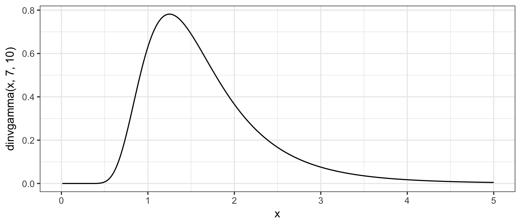
The CDF
can be evaluated with the pinvgamma() function:
f <- function(x) dinvgamma(x, shape, rate)
q <- 2

integrate(f, 0, q)
#  0.7621835 with absolute error < 7.3e-05

(p <- pinvgamma(q, shape, rate))
#  [1] 0.7621835
The quantile
function can be evaluated with qinvgamma():
qinvgamma(p, shape, rate) # = q
#  [1] 2
And random number generation can be performed with
rinvgamma():
set.seed(1234)
rinvgamma(5, shape, rate)
#  [1] 2.640734 1.364965 1.342591 2.095975 1.273201
rinvgamma() can be used to obtain a Monte Carlo
estimate of the probability given by pinvgamma() above:
n <- 1e5
draws <- rinvgamma(n, shape, rate)
mean(draws <= q)
#  [1] 0.76401
Moreover, we can check the consistency and correctness of the implementation with first a kernel density estimate…
plot(density(draws), xlim = c(0,5))
curve(f(x), col = "red", add = TRUE)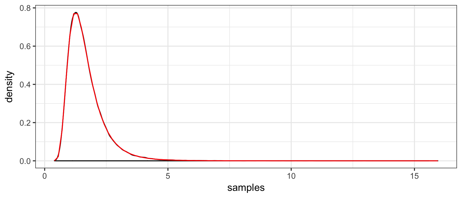
…and also a quantile plot…
qqplot( "x" = ppoints(n) |> qinvgamma(shape, rate), "y" = draws,
  xlab = "Theoretical quantiles", ylab = "Sample quantiles",
  main = "QQ plot for inverse gamma draws"
)
abline(0, 1, col = "red")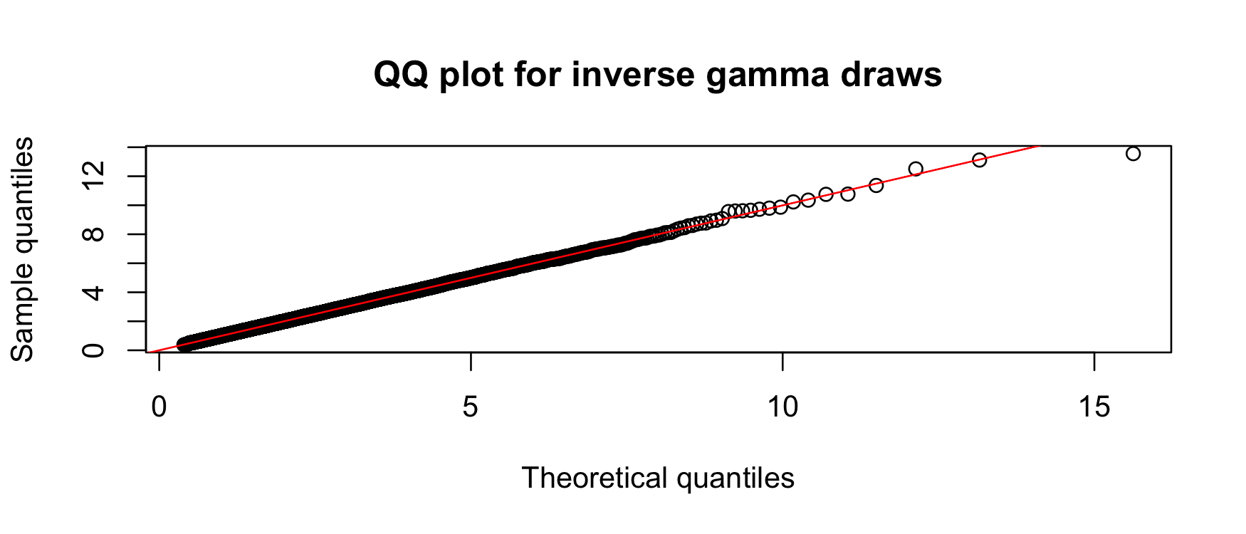
Both of these indicate that the samplers are consistent. As an inferential alternative, we can use a KS test:
ks.test(
  draws,
  function(p) pinvgamma(p, shape, rate)
)
#
#   Asymptotic one-sample Kolmogorov-Smirnov test
#
#  data:  draws
#  D = 0.0029822, p-value = 0.3361
# alternative hypothesis: two-sided[dpqr]invchisq() and [dpqr]invexp()
functionsThe gamma
distribution subsumes the chi-squared
and exponential
distributions,
so it makes sense to include the *invchisq() and
*invexp() functions in invgamma. Their
implementations, however, wrap *chisq() and
*exp(), not *invgamma().
As detailed here, the
parameterizations of the functions in this package cue off of their
corresponding non-inverse distributions from stats.
This commonly causes the confusion that, for example, the parameter
rate in dinvgamma() is the rate parameter of
the inverse gamma distribution. It is not! It is the rate parameter of
the corresponding gamma distribution. Please take care with this
distinction.
invgamma was intended to be a lightweight and simple, largely self-maintaining package implementing the inverse gamma, inverse chi-square, and inverse exponential distributions. It uses the transformation theorem in all cases.
One of the challenges to using naive implementations of distributions is that their numerics may not work well. Arithmetic on a computer is not the same as arithmetic in theory, the kind that you meet in math classes, and as a consequence the best computer implementations of mathematical facts/algorithms need to be tailored to the specific cases at hand.
In January 2023 I did a little poking around into this for
rinvgamma() and found that it performs poorly when the
shape parameter is less than .001 or so. The resulting distributions are
very heavy-tailed, and the draws from these distributions returned by
rinvgamma() are so large that they get rounded to either
very large numbers (where the floating point representation of numbers
does not provide many numbers) or infinity. Here’s an example:
rinvgamma(10, shape = .001, rate = 7)
#  Warning: `rinvgamma()` is unreliable for `shape` <= .01.
#   [1]           Inf           Inf 1.192692e+213           Inf 3.289218e+167
#   [6]           Inf           Inf 7.899428e+197  3.938612e+97           Inf
Notice that rinvgamma() issues a warning in this
circumstance; this is the general behavior of invgamma:
if a particular parameter configuration is known to not produce valid
results, a warning is issued.
rinvgamma()Here is a more detailed Monte Carlo investigation that checks sampler quality using the Kolmogorov-Smirnov test.
First, we write a basic Monte Carlo test for the sampler that works
by generating a large (n = 1e6) sample of draws from the
inverse gamma distribution for a given shape and rate:
test_invgamma <- function(shape, rate, n = 1e5) {
  draws <- rinvgamma(n, shape, rate)
  ks.test(draws, function(p) pinvgamma(p, shape, rate))$p.value
}

test_invgamma(3, 7)
#  [1] 0.3464601
The function returns the \(p\)-value associated with the KS test, so “small” values suggest a departure from the null hypothesis that the distribution is from the corresponding inverse gamma distribution: the sampler is performing poorly. Under the null hypothesis, the \(p\)-value has an approximate uniform distribution, a fact that can be found in most advanced mathematical statistics books, so we would expect some proportion to be small regardless.
We want to see the behavior of the sampler rinvgamma()
across a wide array of parameter values. To do this, we use a range of
parameter values running from small (\(10^-4\)) to large (\(10^4\)):
# load tidyverse and related
library("tidyverse"); library("patchwork"); library("scales", warn.conflicts = FALSE)
theme_set(theme_minimal()); theme_update(panel.grid.minor = element_blank())

# load furrr for parallel computing
library("furrr"); furrr_options(seed = TRUE)
#  <furrr_options>
plan(multisession(workers = parallelly::availableCores()))

# set parameter values to test
n_grid <- 51
param_vals <- 10^seq(-4, 4, length.out = n_grid)
(param_grid <- expand_grid("shape" = param_vals, "rate" = param_vals))
#  # A tibble: 2,601 × 2
#      shape     rate
#      <dbl>    <dbl>
#   1 0.0001 0.0001
#   2 0.0001 0.000145
#   3 0.0001 0.000209
#   4 0.0001 0.000302
#   5 0.0001 0.000437
#   6 0.0001 0.000631
#   7 0.0001 0.000912
#   8 0.0001 0.00132
#   9 0.0001 0.00191
#  10 0.0001 0.00275
#  # ℹ 2,591 more rows
Here’s what the experiment’s design space looks like:
# make axes labeller
fmt <- scales::math_format(10^.x)

# make plot
ggplot(param_grid, aes(shape, rate)) +
  geom_point() +
  scale_x_log10(expression(alpha), n.breaks = 10, labels = fmt(-5:5)) +
  scale_y_log10(expression(lambda), n.breaks = 10, labels = fmt(-5:5)) +
  labs("title" = "Parameter Values at Which to Test `rinvgamma()`") +
  coord_equal()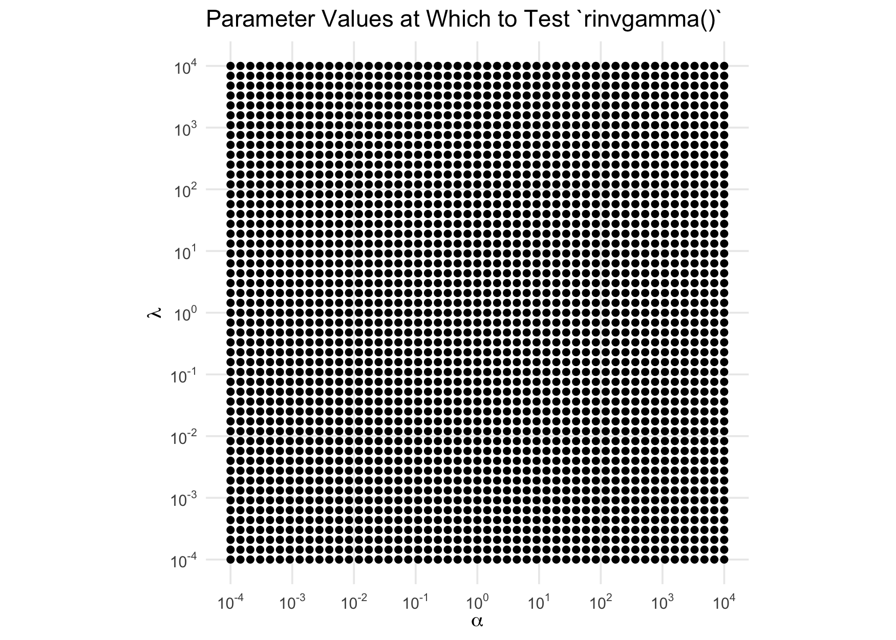
Now, we run our test for each point in the design space in parallel. (Note: we’ve suppressed warnings here that are relevant.)
param_grid <- param_grid |>
  mutate(p_val = future_map2_dbl(shape, rate, test_invgamma))
And we visualize the distribution of the \(p\)-values over that space, binning the colors to at .05 to highlight the rejections of the tests at the 5% level:
ggplot(param_grid, aes(shape, rate, color = p_val)) +
  geom_point() +
  scale_x_log10(expression(alpha), n.breaks = 10, labels = fmt(-5:5)) +
  scale_y_log10(expression(lambda), n.breaks = 10, labels = fmt(-5:5)) +
  scale_color_binned(breaks = c(0, .05, 1)) +
  labs(color = "p value") +
  labs("title" = "KS GoF Test of Draws for Different Parameter Values") +
  coord_equal()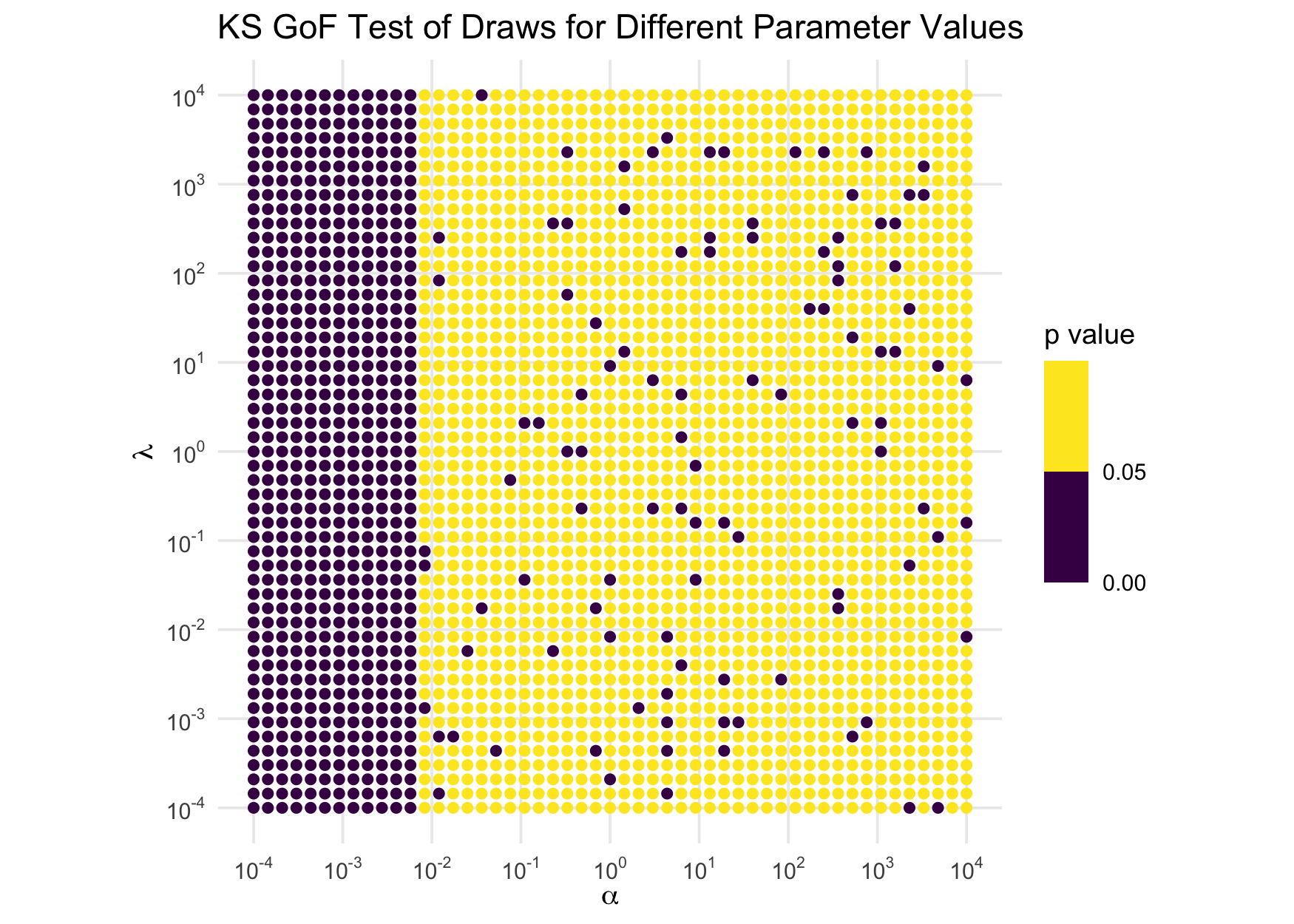
If the sampler were working correctly, the \(p\)-values would be approximately IID
uniform(0,1), so we would expect about 5% of the points to be purple,
and those 5% would be uniformly distributed over the whole space with no
patterns. Obviously, that’s not the case: when the shape parameter is
small, the test is always rejecting. Clearly, when shape is
small, the sampler does not work well. Further investigations reveal
that, as an easy rule, the sampler can be considered unreliable for
shape values less than 0.01. As a consequence,
rinvgamma() issues a warning in those circumstances. (This
warning has been suppressed in the above computations.)
rinvchisq() and
rinvexp()Similar investigations using the inverse chi-squared and inverse
exponential reveal that rinvchisq() should not be trusted
when df <= .01 and ncp <= 10 and
rinvexp() is trustworthy for all values. Here is the
illustration for the inverse chi-squared:
test_rinvchisq <- function(df, ncp, n = 1e5) {
  draws <- rinvchisq(n, df, ncp)
  ks.test(draws, function(p) pinvchisq(p, df, ncp))$p.value
}

expand_grid("df" = param_vals, "ncp" = param_vals) |>
  mutate("p_val" = future_map2_dbl(df, ncp, test_rinvchisq)) |>
  ggplot(aes(df, ncp, color = p_val)) +
    geom_point() +
    scale_x_log10(expression(nu), n.breaks = 10, labels = fmt(-5:5)) +
    scale_y_log10("ncp", n.breaks = 10, labels = fmt(-5:5)) +
    scale_color_binned(breaks = c(0, .05, 1)) +
    labs(color = "p value") +
    coord_equal()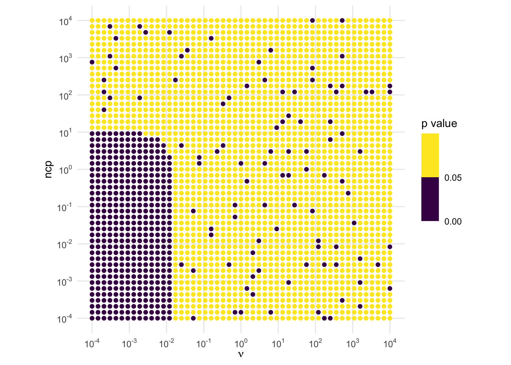
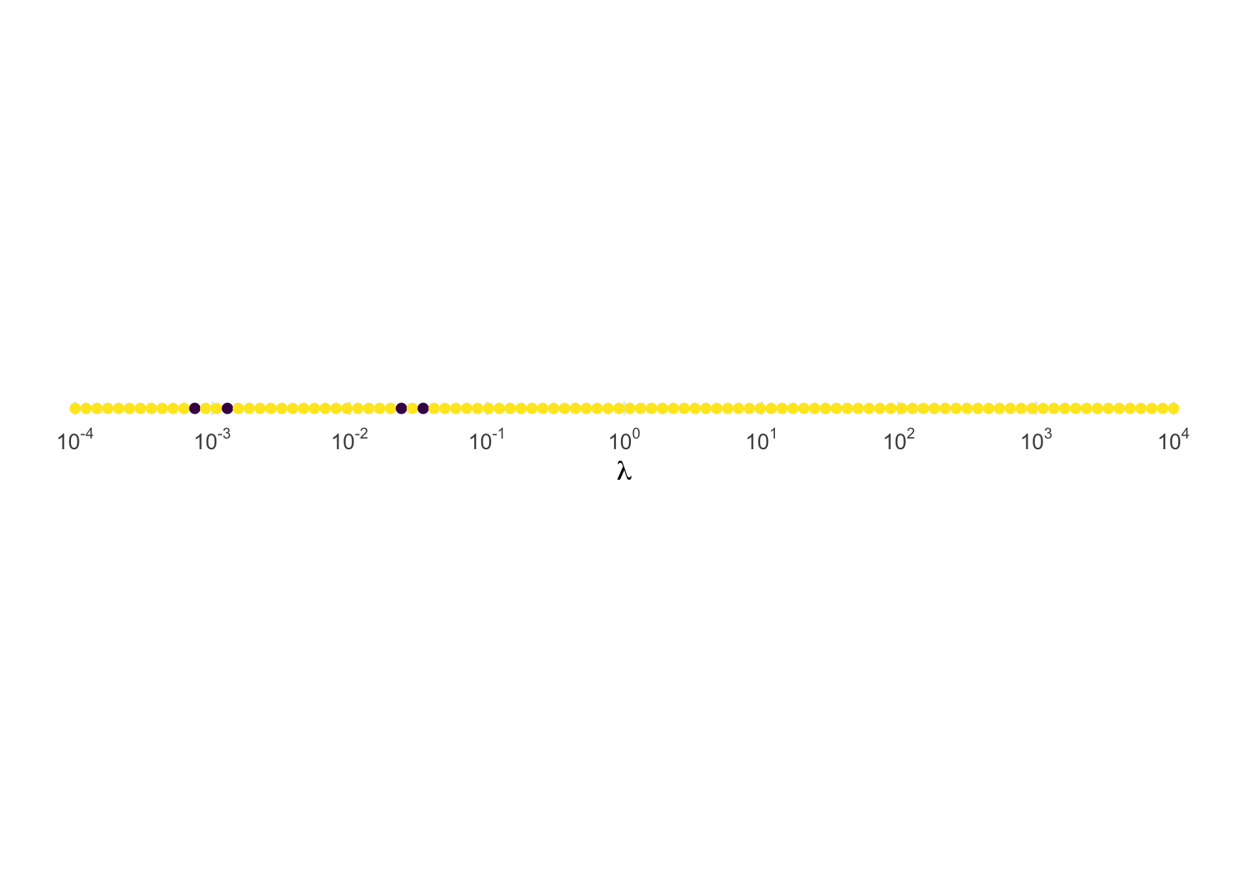
And here is the illustration for the inverse exponential:
test_rinvexp <- function(rate, n = 1e5) {
  draws <- rinvexp(n, rate = rate)
  ks.test(draws, function(p) pinvexp(p, rate))$p.value
}

tibble("rate" = 10^seq(-4, 4, length.out = 2*n_grid)) |>
  mutate("p_val" = future_map_dbl(rate, test_rinvexp)) |>
  ggplot(aes(rate, 0, color = p_val)) +
    geom_point() +
    scale_x_log10(expression(lambda), n.breaks = 10, labels = fmt(-5:5)) +
    scale_color_binned(breaks = c(0, .05, 1), guide = FALSE) +
    theme(axis.text.y = element_blank(), axis.title.y = element_blank(),
          panel.grid.major.y = element_blank()) +
    coord_equal()